Field description

Table 1- Field summary

The field in question (Table 1.) can be considered a moderately sized GAP model, ranging in size between 200 and 700 wells with potentially, millions of feet of multiphase pipelines. The model is required to be run as fully compositional order to generate the required forecast and allow potential optimisations that can be performed on the process system to be evaluated. An added benefit of this can also be seen through the inclusion of flow assurance with the tuned equation of state (EOS), wax/hydrates formation etc.

A number of constraints are present in the system, maximum gas rates and drawdown constraints will be necessary and also potentially fluid velocities in pipelines. Total field rate constraints are also present, creating a convex, non-linear optimisation problem.

The potential to route wells to different manifolds, is also present meaning that in reality a routing optimisation could show potential to significantly enhance production.

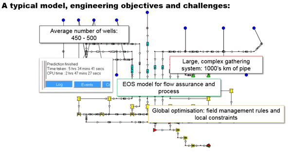
Figure 1 - model setup

Initial status of the model

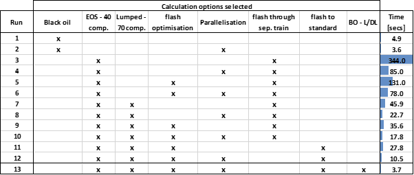
As part of an initial field evaluation this model was built and calibrated using a black oil description of the fluid. Moving to a fully compositional model, naturally showed a significant increase in calculation time. (Table. 2) Run 1 and Run 3 can be seen as a direct comparison between the network solve time of the model using black oil fluid description and the full EOS. It can be seen that the model runs in the order of 70x times slower.

Table 2 - Model calculation time - solve network (no optimisation)

In order to understand the drastic increase in solve time it is important to understand the scope of the problem that is being solved.

Production network modelling

The model that is being solved can be directly compared to another common calculation in the oil industry, e.g. a numerical reservoir model. (Fig. 2)

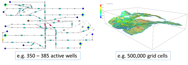
Figure 2 - comparison of two calculations that are similar in scale

In order to compare these two calculations it is important to understand how they are solved and what is necessary to prepare the calculation data for the solvers.

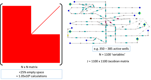
Figure 3 - Preparation of a Jacobian matrix in order to solve the production network model

The model shown in Fig. 3 has around 1100 ‘variables’ these variables represent the pressure drop, rate balance equations in the network. In order to solve this system it is necessary to create a Jacobian of the system, this represents the derivatives every item in the network with respect to every other item, in both rate and pressure. This creates a matrix with roughly 1 million entries calculated, a dense matrix with over 75% filled space.

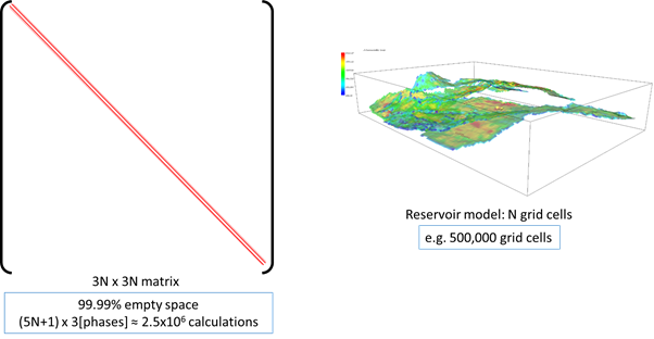
Figure 4 - Numerical reservoir model matrix for calculation

Figure 4 shows a representation of a matrix that is created in order to solve a numerical reservoir model. The diagonal represents the connections between each grid cell and the derivatives of the equations, saturation and pressures of the phases, for each cell. The matrix is larger in sizer with respect to memory (3Nx3N, where N is the number of cells), however the matrix is roughly 99.9% empty (a sparse matrix) meaning that it requires roughly 2.5 million calculations to prepare the data for the solver.

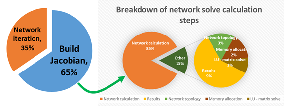
Figure 5 - Building the Jacobian matrix for the network calculation is the most computationally expensive part of the calculation

In order to continue the comparison it is necessary to compare the complexity of the calculations that are required to fill the matrices in Figure 3 & 4. The reservoir model matrix is created using relatively simple linear equations and table lookups to fill in each entry, however in the production network matrix each entry represents a complex calculation, e.g. a full, centre perturbation derivative of an entire pipeline multiphase calculation in both pressure and rate. Meaning that in order to create one entry in the matrix it may be necessary to calculate the pressure drop in a pipeline several miles long roughly 5 times. This results in the generation of this data being the largest part of the total calculation time, around 85% or higher for large models (Fig. 5).

In the case study model, using the full EOS it also requires around 500,000 full flash calculations.

At this point we can also recognise how important the response of the models are, incorrect VLP generation; poor choice of multiphase flow correlation; or, poorly matched EOS can create poor quality derivatives. This will directly impact the quality of the Jacobian and the ability of the matrix solvers to find a valid solution.

Before undertaking and modelling working the model for the study was thoroughly reviewed based on the PE Limited standard recommendations. VLPs were generated using the recommended ranges and the default pipeline model Hydro 2P, is set in each pipeline due to its stability and accuracy as a multiphase flow correlation.

Increasing calculation speed

The ability to parallelise the network calculation in GAP was an enhancement included in IPM 9. This parallelisation is used to generate the Jacobian matrix required for the network calculation. Given the amount of time taken in the total calculation to generate the Jacobian, any saving in time that can be made will have direct benefits to the overall calculation. Figure 6 shows and example of the significant saving in time required to generate the Jacobian for a standard model, we can see the decrease in the time required to build the Jacobian matrix, leading to benefits in the total solve time.

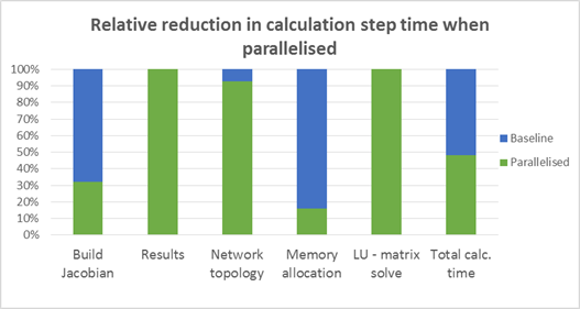
Figure 6 - relative breakdown of timings for different parts of the calculation

In relation to this case study, runs 3 & 4 (Table 2.) show the benefit of using parallelisation. The total calculation time can be seen to reduce by a factor of around 4.

Despite the saving in time this enhancement still leaves the optimisation time for the total model at around 29 minutes for a single full field optimisation. It is therefore necessary to see if the time can be reduced even more.

In IPM 11 an enhancement to the flash calculation speed has been included in all the IPM tools. This enhancement is essentially a simplification to the flash algorithm that enables the tools to skip unnecessary calculations during the flash. This option allows us to further reduce the calculation time, comparing runs 4 & 6 shows roughly a 10% reduction.

Problem formulation to enhance calculation speed

At this stage the model solve time has been reduced to around 22% of the initial solve time when the full composition was included. In order further enhance the calculation time it will be necessary to analyse the reason that the calculation takes so long.

In general, larger compositional models take longer to solve, therefore in order to reduce the calculation time further it is necessary to lower the number of components being used in the flash calculations.

Lumping and de-lumping is a technique that is available in the IPM tools that allows a large composition to be reduced to smaller, and in turn back into larger compositions without losing any information. Reducing the number of components using lumping/de-lumping in the IPM tools further reduces the calculation time from 344 seconds to 17.8 seconds (runs 3 & 10, Table 2. roughly 5% of original solve time).

Process optimization – time saving opportunity

One of the stated objectives of the study is to perform an optimization of the process path the fluid takes. At present the fluid rates are reported through a multistage separation process, this creates a defined GOR, API and gas gravity from the composition that arrives at the separators. Changing the path to surface will change the GOR, API and gas gravity reported and therefore the rates reported.

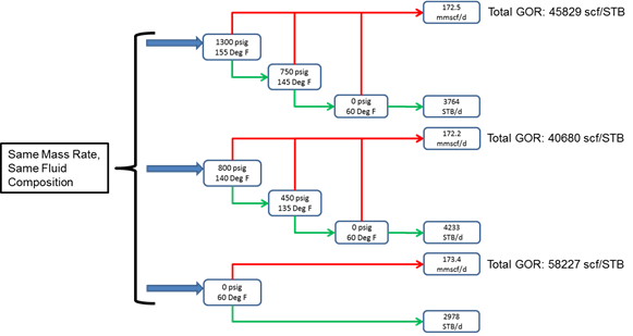
Figure 7 - changing the path to surface for a fluid

Including multistage separation in a flash calculation, however, has a calculation overhead. It is necessary to perform extra flashes through each stage to generate the information for the flash calculations. Therefore removing the multistage flash from the calculation and using a flash straight to stock tank conditions generates a further saving in the calculation time. (Table 2., runs 10 & 12 – 17.8 seconds and 10.5 seconds respectively)

It is important to note that the mass rates that will be used in the network calculations will be identical however the volumetric rates in gas and oil will be different. It is, however, a simple calculation using the Path-to-surface object in RESOLVE. (Fig. 8)

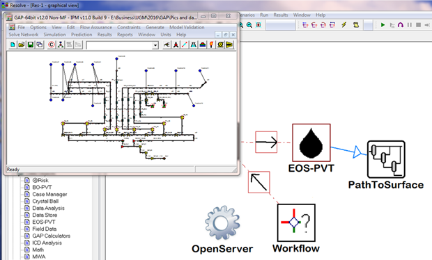
Figure 8 - PathToSurface correction in RESOLVE

An additional saving can be seen outside of the model solve time with this addition to the problem formulation.

In order to perform process optimisation it is necessary to re-generate the well lift curves for each process path. Given that there is almost 300 wells this VLP generation for each process path is an expensive procedure. Using the Path-To-Surface object in RESOLVE (Fig. 8) means that a single set of VLPs can be used for all sensitivities, and in fact a single prediction run can be transformed into multiple sensitivities simply using the composition, the mass rates and the different process paths.

Further network solve speed enhancements

At this stage the network calculation time for a single solve has been taken from 344 seconds down to 10.5 seconds simply using some of the advanced options available in the IPM tools and also some problem formulation, with RESOLVE data objects. The process optimisation can be carried out using only a single model forecast run.

With a network solve time of 10.5 seconds the full field optimisation for the model can be performed in roughly 3.5 minutes, however it is still possible to enhance the speed of the calculations further.

Black oil lumping/delumping is a technique available in GAP which allows the composition to be used in the model to generate fluid properties and blending/separation calculations however it takes advantage of the stability and speed of black oil fluid modelling in any pipeline calculation. Using this option (Run 13, Table 2.) it is possible to bring the network solve time down to around 3.7 seconds without losing any of the calculated results. In fact, each of the runs in Table 2 represent a result with a relative standard deviation of less than 0.5%.

Network solve time and its impact on optimization

At this point the total network optimization time for the model is less than 2 minutes. It is important to understand that the network solve is used to generate information for the optimization, therefore any enhancements that are made in the network solve are also seen in the optimization.

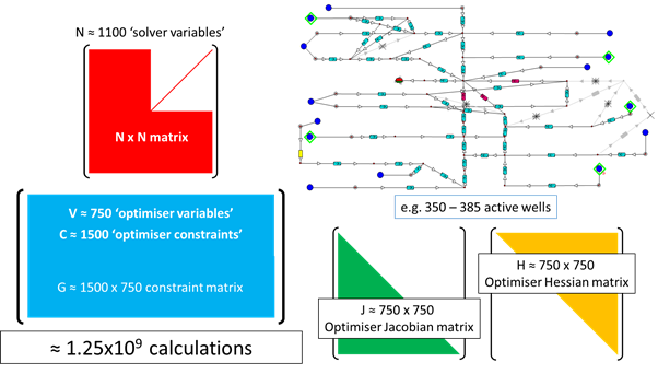
Figure 9 - information required in order to perform a network optimization

Figure 9 shows the information generated in order to perform an iteration of the GAP optimizer. The Jacobian NxN matrix (Fig. 3) is used to generate information for the constraint matrix (G) and the optimizer Jacobian and Hessian matrices. These matrices are compiled for each optimisation control variable and constraint. Each entry in the matrix G is the result of a network calculation performed using the Jacobian matrix, this technique allows a GAP optimisation to be solved in minutes and not in hundreds of days.

Figure 9 also shows how problem formulation can benefit the optimisation even further. Each entry in matrix ‘G’ (the constraint matrix) requires a calculation of the network performance. Therefore ensuring that matrix G is only as small as it needs to be will make the full optimisation even more efficient, since less information is required to be generated for the non-linear optimization algorithm. In general, around 99.8% of the total model optimization time for a GAP optimization is spent generating the information in the schematic in Figure 9, the optimisation algorithm, which is the fastest available today in the industry, takes roughly less than 0.2% of the total calculation time.

In this case study, it is possible to formulate the problem for the optimization of the full field, with tighter solver tolerances for a tighter solution, providing all the required compositional information at around 40 seconds per optimization timestep using a work flow in RESOLVE. This efficiency is brought about through rationalising all of the constraints in the system and guiding the optimizer through a visual workflow at each timestep.

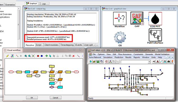
Figure 10 - RESOLVE forecast model - visual workflow and advanced options like parallelisation, PVT flash optimisation and lumping/de-lumping create significant reductions in total calculation time

Conclusions

In this case study the sequential enhancement in speed and efficiency of calculation was demonstrated through use of advanced features in the IPM tool, however more significantly problem formulation was also shown to have an even greater impact in calculation spead.

“A well formulated problem will be solved quickly and efficiently, a poorly formulated problem may not even be solved at all.”